Using Color Surfaces to Incorporate an Identity • colorpath

library("colorpath")
library("purrr")
library("ggplot2")
library("glue")

One goal of this package is to help you design sets of categorical and quantitative palettes that are consistent amongst themselves.

We propose a mechanism for this, what this package calls a surface.

Single-hue surface

At it’s simplest, a surface is the set of all colors (in a given color space) with a given hue. Let’s consider a dark-blue hue in the Jzazbz color-space:

sfc_blue <- pth_new_surface("#0000FF", transformer = pth_to_jzazbz100)

It takes a few seconds for the surface to be computed; it is calculating values for maximum chroma. Here’s a plot of the result:

pth_plot_surface(sfc_blue)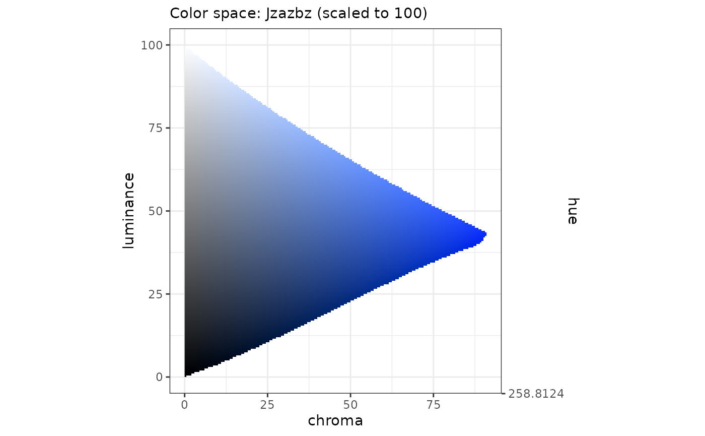

This surface is a slice of the RGB gamut for the Jzazbz color-space (scaled here to 100) where the hue is fixed to the hue of #0000FF.

We can make a similar surface for cyan (#00FFFF):

sfc_cyan <- pth_new_surface("#00FFFF", transformer = pth_to_jzazbz100)
pth_plot_surface(sfc_cyan)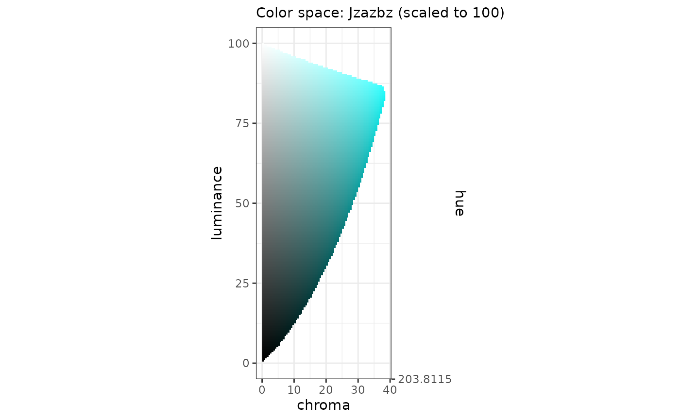

We notice a couple of things here:

the maximum chroma for blue is at a low luminance.
the maximum chroma for cyan is at a high luminance.

Multi-hue surfaces

We can create a surface that captures both these maxima:

sfc_cyan_blue <- pth_new_surface(c("#00FFFF", "#0000FF"), transformer = pth_to_jzazbz100)
pth_plot_surface(sfc_cyan_blue)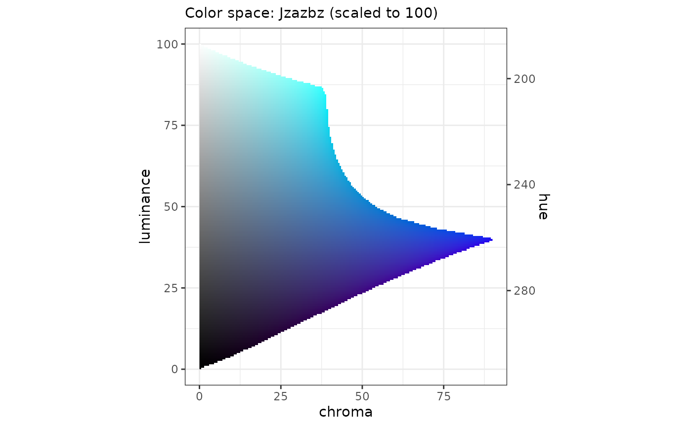

This shows another aspect of surfaces: using the given color-space, hue is a linear function of luminance. This was also the case for the single-hue surfaces.

Also note that you can define surfaces using hex-codes. This could be useful if you are designing a set of palettes for an organization, you can design surfaces using the hex-codes of existing brand-colors.

When you create a surface using hex-codes, you have to specify the color-space to be used; provide a transformer function such as pth_to_jzazbz100, without the parentheses.

There are couple other arguments to pth_new_surface():

use n_step to specify the number of steps, in luminance, to use in calculating the maximum chroma. The max-chroma is calculated once, as the surface is being created; a much quicker approximation-function is used thereafter.
use route to specify if the variation of hue - to we take the "short" (default) or "long" route around the unit circle? The "long" value may be useful if you are designing a surface to build a viridis-like or inferno-like palette.

You can see that the surface sfc_blue_cyan starts to look “purple” for values of luminance below around 40. We can make the surface more “blue” at the low end by choosing a different dark blue, in this case "#000099":

sfc_cyan_blue_clipped <- pth_new_surface(c("#00FFFF", "#000099"), transformer = pth_to_jzazbz100)
pth_plot_surface(sfc_cyan_blue_clipped)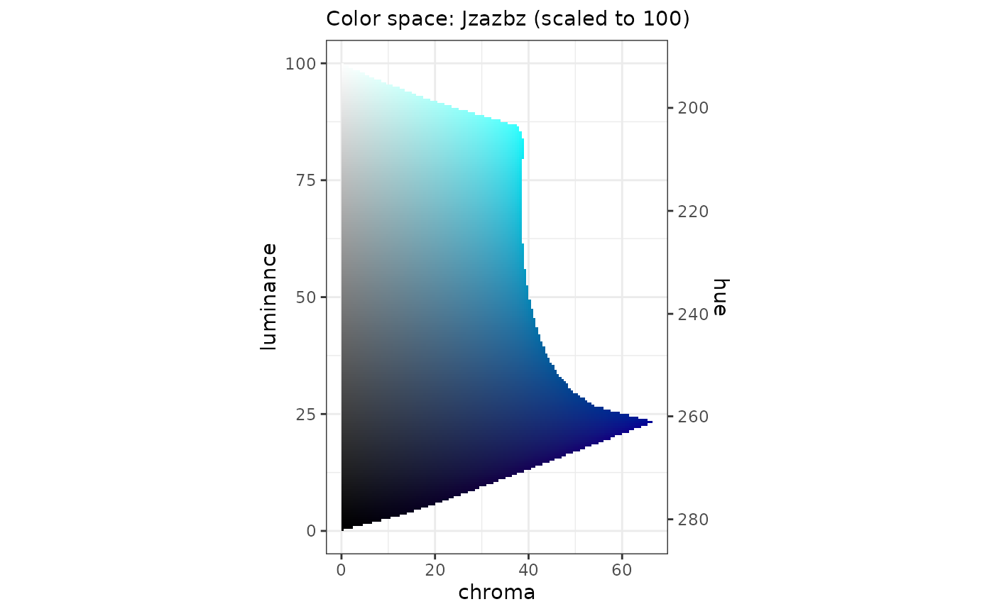

This surface looks more “blue” top-to-bottom.

Incorporating an identity

My suggestion for a set of palettes is to specify four surfaces. In this case, I’ll choose:

a set of blues
a set of oranges
a set of greens
a set of purples

We’ll also look at how these surfaces behave when we simulate color-vision deficiency.

colors <- list(
  blues = c("#42B4E6", "#0087CD"),
  oranges = c("#E47F00", "#702407"),
  greens = c("#007626", "#70E07C"),
  purples = c("#3D1152", "#C530FF")
)

surfaces <- purrr::map(colors, pth_new_surface, transformer = pth_to_jzazbz100)

Here are the surfaces.

I restrained the blues:

pth_plot_surface(surfaces$blues)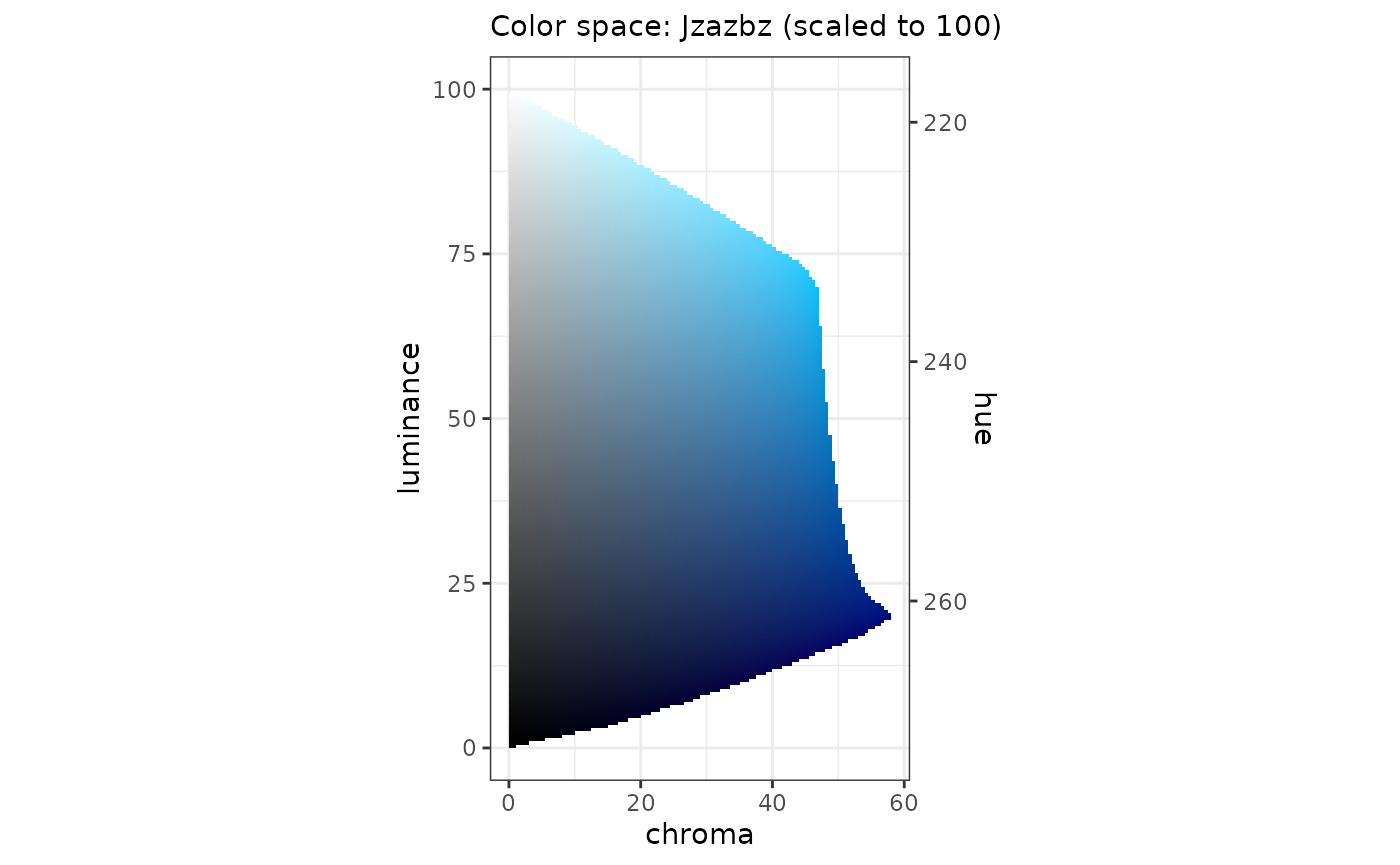

With the oranges, I added a redder-orange with lower luminance to add some chroma to the lower “half” of the luminance range.

pth_plot_surface(surfaces$oranges)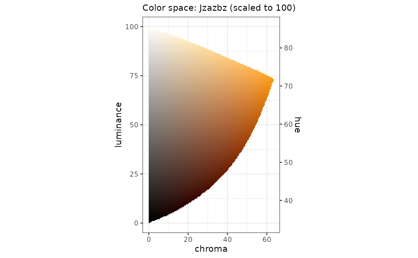

Whereas the blues and oranges are multi-hue the greens and purples are more single-hue:

pth_plot_surface(surfaces$greens)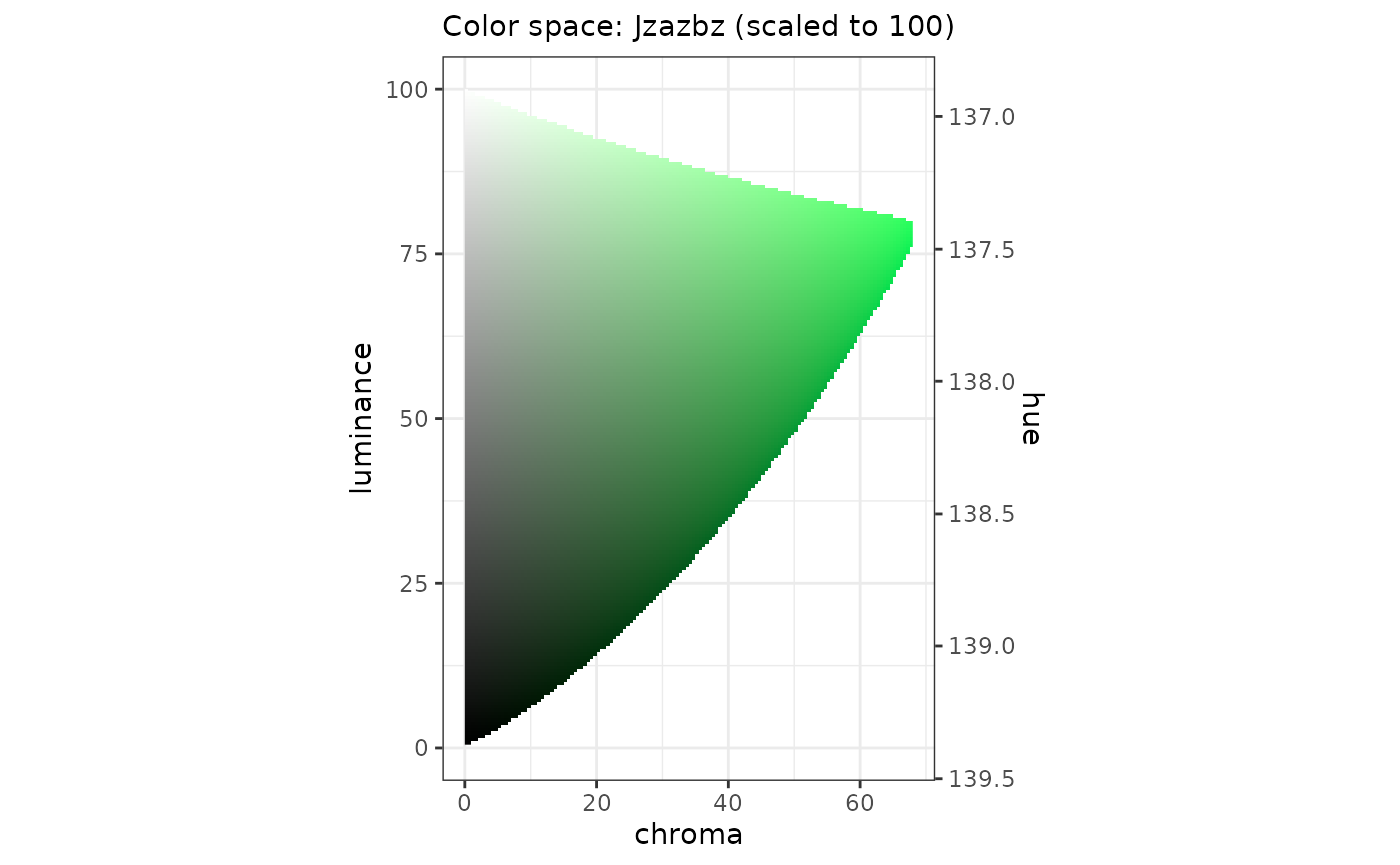

pth_plot_surface(surfaces$purples)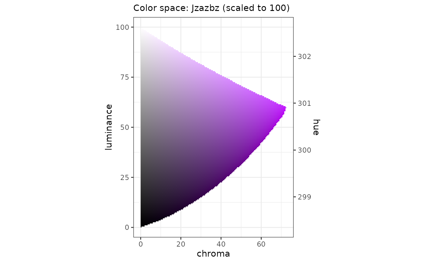

Color-vision deficiency

The idea is that all the colors used in a set of categorical and quantitative palettes would be found on these surfaces. It could be useful to see how these surfaces interact with each other under simulated color-vision deficiency (CVD).

Our first step is to generate lots of colors. Here, for each of our surfaces, we are generating (in this case 21) colors at the maximum-chroma, distributed evenly along the luminance domain.

mat_surfaces <- 
  surfaces %>%
  map(pth_mat_max_chroma) %>%
  reduce(rbind)

Next, we can plot these colors in polar coordinates, using pth_plot_polar():

pth_plot_polar(mat_surfaces, cvd = pth_cvd_grid_full()) +
  facet_grid(
    rows = vars(condition), 
    cols = vars(severity),
    labeller = labeller(severity = label_both)
  ) +
  ggtitle(
    label = "Outer (chroma) edge of surfaces, simulating color-vision deficiency",
    subtitle = glue("Color space: {pth_colorspace_name(mat_surfaces)}")
  )

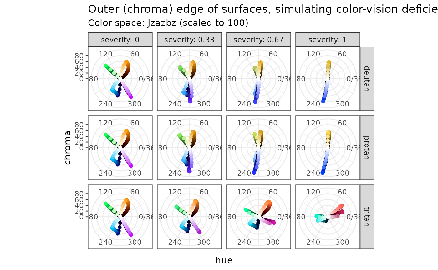
This is a facetted plot. Each row shows a given type of color-vision deficiency (deutan is most prevalent); each column shows a certain severity.

We are plotting points that lie on the most-chromatic part of each surface; this can give us an idea of how that surface behaves within the color space. We can use this mental-model as a guide to untangle color “collisions” in CVD. Keep in mind that the points are equally-spaced in luminance, the luminance considered in the non-CVD case.

In each case, the color space collapses from three to (almost) two dimensions. However, in each case, blues are always opposite to oranges; greens are always opposite to purples.

Next steps

We will use these surfaces as the bases for categorical and quantitative palettes, for both light mode and dark mode. Our design constraints will also include the background color we will use for both light mode and dark mode.